Distribuciones & LogNorm
09 Jul 2015Como explicavamos en Initial Exploration, las rows de las diferentes tablas son tipo la siguiente:
| zipcode | date | category | merchant | card | payment | avg | max | min | std | |
|---|---|---|---|---|---|---|---|---|---|---|
| 33 | 8001 | 2014-07-04 | es_barsandrestaurants | 89 | 447 | 457 | 25.51 | 187 | 1.1 | 23.913212 |
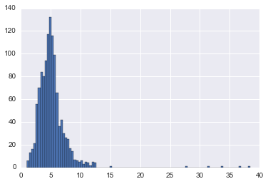
en concreto para la basic_stats, tenemos para cada Zipcode, date, category los parametros de "una" distribución, avg, max, min y std. Despues de analizar los datos podemos suponer que una distribución que se adapta bien es la LogNorm:
$$ f(x~|~\mu, \sigma) = \dfrac{1}{x\sigma\sqrt{2\pi}} e ^{ \dfrac{-(lnx - \mu)^2}{2\sigma^2} } $$
https://en.wikipedia.org/wiki/Log-normal_distribution
scipy.stats nos proporciona la siguiente función:
http://docs.scipy.org/doc/scipy-0.15.1/reference/generated/scipy.stats.lognorm.html
$$ f(x~|~\textbf{[shape]}, \textbf{[location]}, \textbf{[scale]}) = \dfrac{1}{(x-\textbf{[location]})\textbf{[shape]}\sqrt{2\pi}} e ^{ \dfrac{-(ln(x-\textbf{[location]})-ln(\textbf{[scale]}))^2}{2\textbf{[shape]}^2}} $$
despues de intentar ver como adaptar nuestros parametros sin exito, vemos que es algo común:
http://nbviewer.ipython.org/url/xweb.geos.ed.ac.uk/~jsteven5/blog/lognormal_distributions.ipynb
http://stackoverflow.com/questions/15630647/fitting-lognormal-distribution-using-scipy-vs-matlab
http://stackoverflow.com/questions/18534562/scipy-lognormal-fitting
http://stackoverflow.com/questions/8747761/scipy-lognormal-distribution-parameters
http://broadleaf.com.au/resource-material/lognormal-distribution-summary/
asi que despues de ponerlo todo en común, y operando obtenemos:
para nuestros datos en concreto, definimos la siguiente función:
def LogNormbyAvgStdNum(row):

    avg=row["avg"]
    std=row["std"]
    num=row["payment"]

    var=std*std
    sigma2=np.log(1+(var/(avg*avg)))
    sigma =np.sqrt(sigma2)
    mu = np.log(avg)-(.5*sigma)

    r = lognorm.rvs(sigma, loc=0,scale=np.exp(mu), size=num)
    return r
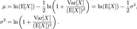
obteniendo, un generador de transacciones, para todas las tablas, un ejemplo de generación:
fig, ax = plt.subplots(1, 1)
ax.hist(LogNormbyAvgStdNum(row),  bins=100, histtype='stepfilled', color='black', alpha=0.2)
ax.hist(LogNormbyAvgStdNum(row_male),  bins=100, histtype='stepfilled', color='blue', alpha=0.3)
ax.hist(LogNormbyAvgStdNum(row_female),  bins=100, histtype='stepfilled', color='red', alpha=0.3)
ax.hist(LogNormbyAvgStdNum(row_enterprise),  bins=100, histtype='stepfilled', color='yellow', alpha=0.3)

plt.show()
podemos añadir una nueva columna con una "muestra" de la distribución:
cut100_gender_distribution_restaurants=gender_distribution_restaurants[:100]
cut100_gender_distribution_restaurants["distribution"] = ""
for i in cut100_gender_distribution_restaurants.index:
    cut100_gender_distribution_restaurants["distribution"][i] = LogNormbyAvgStdNum(cut100_gender_distribution_restaurants.ix[i])
| zipcode | date | category | gender | other columns | distribution | |
|---|---|---|---|---|---|---|
| 8 | 8001 | 2014-07-27 | es_barsandrestaurants | female | ... | [43.1818628059, 29.9470395686, 14.3600232708, ... |
| 15 | 8001 | 2014-07-10 | es_barsandrestaurants | female | ... | [13.1878541979, 80.1620829974, 9.70680394996, ... |
| ... | ||||||
| 623 | 8018 | 2014-07-16 | es_barsandrestaurants | female | ... | [16.2716453202, 13.056585559, 10.8981710228, 1... |
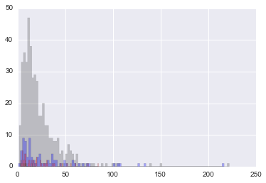
total= np.hstack(basic_stats_restaurants_08001["distribution"])


fig, ax = plt.subplots(1, 1)
ax.hist(total, bins=100, histtype='stepfilled',  alpha=0.5)
plt.show()
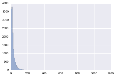
de forma inversa podemos intentar ver la distribución merchants, payments, cards, avgpaybymerch, amountbymerch:
| zipcode | date | category | gender | merchant | card | payment | avg | max | min | std | |
|---|---|---|---|---|---|---|---|---|---|---|---|
| 22494 | 8001 | 2014-07-04 | es_barsandrestaurants | unknown | 27 | 303 | 309 | 25.51 | 118.75 | 1.1 | 19.952131 |
| 53924 | 8001 | 2014-07-04 | es_barsandrestaurants | female | 41 | 53 | 55 | 24.57 | 137.60 | 3.0 | 22.800214 |
| 67406 | 8001 | 2014-07-04 | es_barsandrestaurants | male | 53 | 77 | 79 | 29.15 | 187.00 | 3.0 | 36.303650 |
| 72030 | 8001 | 2014-07-04 | es_barsandrestaurants | enterprise | 7 | 14 | 14 | 8.62 | 27.25 | 1.6 | 6.107891 |
por ejemplo:
plt.hist(restaurants_bcn["avgpaybymerch"],bins=100)
References:
http://nbviewer.ipython.org/url/xweb.geos.ed.ac.uk/~jsteven5/blog/lognormal_distributions.ipynb
http://stackoverflow.com/questions/15630647/fitting-lognormal-distribution-using-scipy-vs-matlab
http://stackoverflow.com/questions/18534562/scipy-lognormal-fitting
http://stackoverflow.com/questions/8747761/scipy-lognormal-distribution-parameters
http://broadleaf.com.au/resource-material/lognormal-distribution-summary/